import numpy as np
import matplotlib.pyplot as plt

from boreflow import BCArray, Geometry, Simulation, Flux, Limiter, TimeIntegrationSimulating Custom Flow
Example of simulating custom flow on a horizontal surface and a steep slope.
# 1) Create geometry
x = np.array([0, 2, 11])  # X-coordinate x[i]
z = np.array([3, 3, 0])  # Elevation z[i] at x[i]
n = np.array([0.0175, 0.0175])  # Manning roughness (n) between x[i] and x[i+1]
geometry = Geometry(x, z, n)

# Plot the geometry
plt.figure()
plt.plot(x, z, color="black", label="Geometry")
plt.plot([x[0]], [z[0]], "o", color="red", label="Inflow")
plt.plot([x[-1]], [z[-1]], "o", color="blue", label="Free outflow")
plt.legend()
plt.xlabel("x-coordinate [m]")
plt.ylabel("z-coordinate [m]")
plt.axis("equal")
plt.show()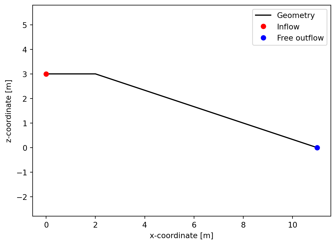
# 2) Create boundary conditions
t = np.array([0, 1, 4])
h = np.array([0.5, 0.8, 0])
u = np.array([1.0, 2.0, 0])
bc = BCArray(t, h, u)

# 3) Initialize simulation settings
sim = Simulation(t_end=10.0, cfl=0.2, max_dt=0.01, nx=110)

# 4) Run the simulation
results = sim.run(geometry, bc, Limiter.minmod, Flux.HLL, TimeIntegration.EF)
Simulating: 0%| | 0.00/10.00 sSimulating: 2%|▏ | 0.15/10.00 sSimulating: 3%|▎ | 0.30/10.00 sSimulating: 4%|▍ | 0.44/10.00 sSimulating: 6%|▌ | 0.58/10.00 sSimulating: 7%|▋ | 0.71/10.00 sSimulating: 8%|▊ | 0.84/10.00 sSimulating: 10%|▉ | 0.96/10.00 sSimulating: 11%|█ | 1.09/10.00 sSimulating: 12%|█▏ | 1.20/10.00 sSimulating: 13%|█▎ | 1.31/10.00 sSimulating: 14%|█▍ | 1.42/10.00 sSimulating: 15%|█▌ | 1.52/10.00 sSimulating: 16%|█▌ | 1.61/10.00 sSimulating: 17%|█▋ | 1.71/10.00 sSimulating: 18%|█▊ | 1.80/10.00 sSimulating: 19%|█▉ | 1.88/10.00 sSimulating: 20%|█▉ | 1.96/10.00 sSimulating: 20%|██ | 2.04/10.00 sSimulating: 21%|██ | 2.12/10.00 sSimulating: 22%|██▏ | 2.20/10.00 sSimulating: 23%|██▎ | 2.27/10.00 sSimulating: 23%|██▎ | 2.34/10.00 sSimulating: 24%|██▍ | 2.41/10.00 sSimulating: 25%|██▍ | 2.47/10.00 sSimulating: 25%|██▌ | 2.54/10.00 sSimulating: 26%|██▌ | 2.61/10.00 sSimulating: 27%|██▋ | 2.67/10.00 sSimulating: 27%|██▋ | 2.74/10.00 sSimulating: 28%|██▊ | 2.80/10.00 sSimulating: 29%|██▊ | 2.86/10.00 sSimulating: 29%|██▉ | 2.92/10.00 sSimulating: 30%|██▉ | 2.98/10.00 sSimulating: 30%|███ | 3.05/10.00 sSimulating: 31%|███ | 3.11/10.00 sSimulating: 32%|███▏ | 3.17/10.00 sSimulating: 32%|███▏ | 3.24/10.00 sSimulating: 33%|███▎ | 3.30/10.00 sSimulating: 34%|███▎ | 3.36/10.00 sSimulating: 34%|███▍ | 3.43/10.00 sSimulating: 35%|███▍ | 3.49/10.00 sSimulating: 36%|███▌ | 3.56/10.00 sSimulating: 36%|███▋ | 3.63/10.00 sSimulating: 37%|███▋ | 3.69/10.00 sSimulating: 38%|███▊ | 3.76/10.00 sSimulating: 38%|███▊ | 3.83/10.00 sSimulating: 39%|███▉ | 3.90/10.00 sSimulating: 40%|███▉ | 3.97/10.00 sSimulating: 40%|████ | 4.04/10.00 sSimulating: 41%|████ | 4.11/10.00 sSimulating: 42%|████▏ | 4.18/10.00 sSimulating: 43%|████▎ | 4.26/10.00 sSimulating: 43%|████▎ | 4.33/10.00 sSimulating: 44%|████▍ | 4.40/10.00 sSimulating: 45%|████▍ | 4.48/10.00 sSimulating: 46%|████▌ | 4.56/10.00 sSimulating: 46%|████▋ | 4.64/10.00 sSimulating: 47%|████▋ | 4.72/10.00 sSimulating: 48%|████▊ | 4.80/10.00 sSimulating: 49%|████▉ | 4.88/10.00 sSimulating: 50%|████▉ | 4.96/10.00 sSimulating: 50%|█████ | 5.05/10.00 sSimulating: 51%|█████▏ | 5.14/10.00 sSimulating: 52%|█████▏ | 5.22/10.00 sSimulating: 53%|█████▎ | 5.32/10.00 sSimulating: 54%|█████▍ | 5.41/10.00 sSimulating: 55%|█████▍ | 5.50/10.00 sSimulating: 56%|█████▌ | 5.59/10.00 sSimulating: 57%|█████▋ | 5.70/10.00 sSimulating: 58%|█████▊ | 5.80/10.00 sSimulating: 59%|█████▉ | 5.91/10.00 sSimulating: 60%|██████ | 6.02/10.00 sSimulating: 61%|██████▏ | 6.14/10.00 sSimulating: 63%|██████▎ | 6.26/10.00 sSimulating: 64%|██████▍ | 6.38/10.00 sSimulating: 65%|██████▌ | 6.51/10.00 sSimulating: 66%|██████▋ | 6.65/10.00 sSimulating: 68%|██████▊ | 6.79/10.00 sSimulating: 69%|██████▉ | 6.94/10.00 sSimulating: 71%|███████ | 7.10/10.00 sSimulating: 73%|███████▎ | 7.26/10.00 sSimulating: 74%|███████▍ | 7.42/10.00 sSimulating: 76%|███████▌ | 7.60/10.00 sSimulating: 78%|███████▊ | 7.79/10.00 sSimulating: 80%|███████▉ | 7.98/10.00 sSimulating: 82%|████████▏ | 8.19/10.00 sSimulating: 84%|████████▍ | 8.41/10.00 sSimulating: 86%|████████▋ | 8.63/10.00 sSimulating: 88%|████████▊ | 8.85/10.00 sSimulating: 91%|█████████ | 9.09/10.00 sSimulating: 93%|█████████▎| 9.33/10.00 sSimulating: 96%|█████████▌| 9.58/10.00 sSimulating: 99%|█████████▊| 9.85/10.00 sSimulating: 100%|██████████| 10.00/10.00 sSimulation done in 9.75 sec# Plot peak flow velocity, peak flow thickness, peak flow discharge
fig, (ax0, ax1, ax2) = plt.subplots(1, 3, figsize=[8, 3.5])
# Mark the transition between the horizontal surface and the sloped surface (x = 2m / s = 2m)
[ax.axvline(2.0, color="grey", ls=":") for ax in [ax0, ax1, ax2]]
# Get results and plot peak flow characteristics
h, u, q = results.get_peak_flow()
ax0.plot(results.s, h, color="black")
ax1.plot(results.s, u, color="black")
ax2.plot(results.s, q, color="black")
# Plot layout
[ax.set_xlabel("Distance (s-coordinate) [m]") for ax in [ax0, ax1, ax2]]
ax0.set_ylabel("Peak flow thickness [m]")
ax1.set_ylabel("Peak depth-avg flow velocity [m/s]")
ax2.set_ylabel("Peak flow discharge [m2/s]")
[ax.set_xlim(0, np.max(results.s)) for ax in [ax0, ax1, ax2]]
[ax.set_ylim(0, None) for ax in [ax0, ax1, ax2]]
fig.suptitle("Peak Flow Characteristics along Geometry")
fig.tight_layout()
plt.show()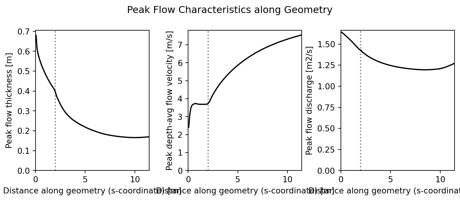
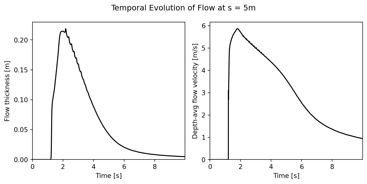
# Plot
fig, (ax0, ax1) = plt.subplots(1, 2, figsize=[8, 4])

# Get and plot the flow at s=5m
res_t, res_h, res_u = results.get_st(s=5.0)
ax0.plot(res_t, res_h, color="black")
ax1.plot(res_t, res_u, color="black")

# Plot layout
[ax.set_xlabel("Time [s]") for ax in [ax0, ax1]]
ax0.set_ylabel("Flow thickness [m]")
ax1.set_ylabel("Depth-avg flow velocity [m/s]")
[ax.set_xlim(0, np.max(res_t)) for ax in [ax0, ax1]]
[ax.set_ylim(0, None) for ax in [ax0, ax1]]
fig.suptitle("Temporal Evolution of Flow at s = 5m")
fig.tight_layout()
plt.show()